This week, we are getting to the topic of Learning Rates for Stable Diffusion fine-tuning, and this time we want to share something more exciting compared to our previous brute-force methods of experimenting with Learning rates (link to the older post).
A few weeks ago, EveryDream trainer added support to the validation process (link). And this enabled the community to apply some of the common Machine Learning approaches to find optimal parameters for the training process.
A couple of users from the ED community have been suggesting approaches to how to use this validation tool in the process of finding the optimal Learning Rate for a given dataset and in particular, this paper has been highlighted (Cyclical Learning Rates for Training Neural Networks). Special shoutout to user damian0815#6663 who has been pioneering the implementation of the validation methodology as well as suggested how to apply this LR discovery method. Check his comments on ED Discord or check out his Github for some useful tools (link).
Please note that the paper is from 2017(!) and a lot of progress has been made in this space since then but nevertheless, there are two interesting concepts there that we can apply to the fine-tuning process. And so far the results that we have been observing are amazing!
The two concepts are 1 - finding the learning rate range and 2 - applying the idea of cyclical learning rates. Today we will discuss the first one (useful on its own) and in the next post, we will try implementing the cyclical approach.

Overview of the Approach to Find LR Range
From the above paper, we read:
There is a simple way to estimate the reasonable minimum and maximum boundary values with one training run of the network for a few epochs. … run your model for several epochs while letting the learning rate increase linearly between low and high LR values. … Note the learning rate value when the accuracy starts to increase and when the accuracy slows, becomes ragged, or starts to fall. These two learning rates are good choices for bounds;
Basically, we do a test run where we gradually increase the learning rate from a very low value (0 works well here) to something that we know is definitely high and watch when the model ‘starts learning’ and then ‘stops learning’. In our case, instead of accuracy, we will use the loss values from the validation process meaning that the graph will be reversed when compared to the above-mentioned accuracy graph: we need to watch the learning rates at the moment when loss values start to go down and when it starts to go back up.
These two values will serve as upper and lower bounds of reasonable learning rates. In theory, anything in-between can be used and the model should be able to learn. Obviously, there are some tradeoffs here - using the lowest value will likely require a higher number of epochs/steps, and using higher values can “bake” the model relatively fast.
Once we know the upper and lower bounds of the learning rates, we can apply them to the fine-tuning process in a few ways. If we want to simply use a constant learning rate then picking a mid-point between the two sounds reasonable. And if we want to do something fancier - now we have bounds of learning rates between which we can alternate.
Our Experiment Setup
All this sounded exciting, we were seeing some great results being shared so we decided to give it a try. We experimented with two datasets, of course with Damon Albarn’s face and also with our previous dataset when we did style experiments. For Damon’s face, we used the cropped training data (link to the older post) just to have a bit more control over the number of steps per epoch, and for style, we used short captions version of the images (link).
You can see the full configs we used at the bottom of the post but here are the key things that were changed for the first run of face training:
- "lr": 3e-06, (basically a value that we know is definitely too high)
- "lr_scheduler": "linear", (to allow a gradual increase in the learning rate)
- "max_epochs": 100, (since our data was just 20 images)
- "lr_warmup_steps": 400, (set this amount to the total number of steps you’ll have, details below. This allows the linear scheduler to go up instead of down).
And of course, validation was enabled at every 1 epoch with the split proportion of 0.2. (full set at the end of the post).
To get intuition on the numbers here let’s discuss a few calculations. "val_split_proportion": 0.2 means that 20% of the data will be split from the dataset, will not be used in the training process and instead it will be used for validation purpose. Since we had 20 images, this means we have 16 images left.
You can calculate the total steps in the training process as the number of images in your dataset * max_epoch and / batch_size. In this case 16*100/4=400. That is why we set lr_warmup_steps to 400, meaning that the learning rate will go from 0 to the set value of 3e-06 in 400 steps while increasing linearly.
Initial Findings for Learning Rates
After the first run with Damon’s data, we got these two graphs:

As expected, the learning rate has been increasing in a linear manner from 0 to 3e-06 over 400 steps. And on the validation loss graph, we see the expected behavior, the model started reducing the loss, then it flattened and finally started to go up.
In theory, we could already derive the values from this graph but we decided to do one more run to zoom in since we saw that at the mid-point the graph already started to flatten and then go up.
So we only changed "lr" to 1.5e-06 (ie we reduced it 2x meaning that the linear increase will be 2x slower) and rerun the experiment.
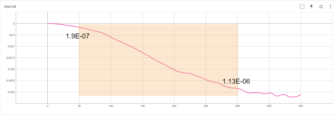
We observe that model started reducing the loss almost immediately so very low learning rates are still training the model and at around 300-350 steps the curve started flattening. We decided to use the lower and upper ranges and 50 and 300 steps respectively getting us values of lower bound: 1.9E-07 and upper bound of 1.13E-06.
Applying Findings - Deciding on the Number of Steps
Now that we have the range of learning rates, we need to figure out how to apply the findings. In the next post, we will discuss a cyclical approach but for now, let’s keep using linear learning rates. To do so, we simply decided to use the mid-point calculated as (1.9E-07 + 1.13E-06) / 2 = 6.6E-07.
The next question after having the learning rate is to decide on the number of training steps or epochs. And once again, we decided to use the validation loss readings. The idea was to run a model at the discovered learning rate of 6.6E-07 for longer than the usually needed steps, check the loss graphs, and see values where the graph flattens and starts to go up. So we changed the lr_scheduler to constant, max_epochs to 200, and of course lr to 6.6E-07. As a result, we got the following graph:

In this case, we decided that somewhere 225-400 total steps model should be optimally trained. One can stop here, get the checkpoints from this range and test the output to confirm a successful fine-tuning.
However, we decided to go a step further given that we had an extra small dataset, and redid the training with validation disabled. Please note that this is a risky step since we are ‘blind’ without validation enabled and we have no idea how exactly those added-back images impact our training process. With the sufficiently large dataset, we recommend skipping this step. And just to confirm the issue, we can compare the stabilize-train loss graphs with 16 and all 20 images and we see that the two diverge further confirming the danger of this approach.
However, we decided to go a step further given that we had an extra small dataset, and redid the training with validation disabled. Please note that this is a risky step since we are ‘blind’ without validation enabled and we have no idea how exactly those added-back images impact our training process. With the sufficiently large dataset, we recommend skipping this step. And just to confirm the issue, we can compare the stabilize-train loss graphs with 16 and all 20 images and we see that the two diverge further confirming the danger of this approach.

Anyways, for the final run we did 110 epochs with validation disabled, and here are the outputs from the model. We feel pretty good about the model, it feels both flexible and accurate.


Validating Finding with Style Training
To ensure it was not a random fluke, we re-run the whole thing for style training. For start we found the LR range:

Then picked the midpoint (5.6E-07) and ran a long training to make a decision on the total steps:

And did the final run at 500 steps (or 50 epochs in this case). Here are some of the results:


Configs Used for The First Run
I’d suggest changing the "log_step" to 1 for more detailed reports, we just forgot here.
{
  "config": "train.json",
  "amp": true,
  "batch_size": 4,
  "ckpt_every_n_minutes": null,
  "clip_grad_norm": null,
  "clip_skip": 0,
  "cond_dropout": 0.04,
  "data_root": "D:\\ED2\\EveryDream2trainer\\input\\...",
  "disable_textenc_training": false,
  "disable_xformers": false,
  "flip_p": 0.0,
  "gpuid": 0,
  "gradient_checkpointing": true,
  "grad_accum": 1,
  "logdir": "logs",
  "log_step": 25,
  "lowvram": false,
  "lr": 3e-06,
  "lr_decay_steps": 0,
  "lr_scheduler": "linear",
  "lr_warmup_steps": 400,
  "max_epochs": 100,
  "notebook": false,
  "optimizer_config": "optimizer.json",
  "project_name": "lr_discovery_2",
  "resolution": 512,
  "resume_ckpt": "sd_v1-5_vae",
  "run_name": null,
  "sample_prompts": "sample_prompts.txt",
  "sample_steps": 300,
  "save_ckpt_dir": null,
  "save_ckpts_from_n_epochs": 0,
  "save_every_n_epochs": 20,
  "save_optimizer": false,
  "scale_lr": false,
  "seed": 555,
  "shuffle_tags": false,
  "validation_config": "validation_default.json",
  "wandb": false,
  "write_schedule": false,
  "rated_dataset": false,
  "rated_dataset_target_dropout_percent": 50,
  "zero_frequency_noise_ratio": 0.02,
  "save_full_precision": false,
  "disable_unet_training": false,
  "rated_dataset_target_dropout_rate": 50,
  "disable_amp": false,
  "useadam8bit": false
}
and validation_default.json settings:
 "validate_training": true,
    "val_split_mode": "automatic",
    "val_data_root": null,
    "val_split_proportion": 0.2,
    "stabilize_training_loss": true,
    "stabilize_split_proportion": 0.2,
    "every_n_epochs": 1,
    "seed": 555